Monte Carlo Simulation

One of the most compelling additions to your analytical arsenal can be the integration of Python in Excel, especially for conducting Monte Carlo simulations. Let’s dive into how this powerful combination simplifies complex financial analyses and brings clarity to uncertainty.

Understanding Monte Carlo Simulations

At its core, a Monte Carlo Simulation is a method to understand the impact of risk and uncertainty in financial models. It might sound like a complex statistical tool, but it's essentially about running multiple scenarios (or ‘simulations’) to predict a range of possible outcomes. Think of it as testing different financial roads to see where each might lead, considering the unpredictability of factors like market conditions, interest rates, or investment returns.

Why Monte Carlo Simulation in Excel with Python?

Traditionally, financial modeling in Excel has limitations, especially when dealing with complex simulations. This is where Python, with its robust libraries and efficient computation capabilities, becomes a game-changer. By integrating Python into Excel, you can perform sophisticated analyses like Monte Carlo simulations more efficiently and accurately.

A Practical Scenario: Revenue Forecasting

Imagine you’re tasked with forecasting next year’s revenue. There are assumptions like expected growth rate and volatility, but how do you account for the inherent uncertainties in these predictions?

This is where a Monte Carlo Simulation comes into play. By running thousands of simulations, each applying random variations to your growth rate within its expected volatility, Python generates a range of possible outcomes. This provides a more comprehensive view of potential future revenues, rather than a single, static prediction.

Implementing the Simulation in Excel with Python

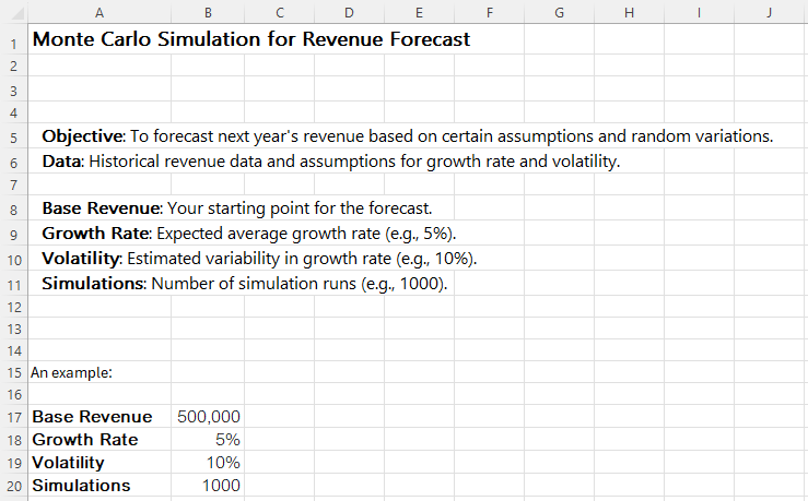
With Python in Excel, you begin by setting your base assumptions directly in an Excel sheet – base revenue, expected growth rate, volatility, and the number of simulations. Using Python, you automate the process of generating random growth rates and applying them to your base revenue to forecast multiple outcomes.

Let's use the example below:

Now we'll add the script in the PY() function:

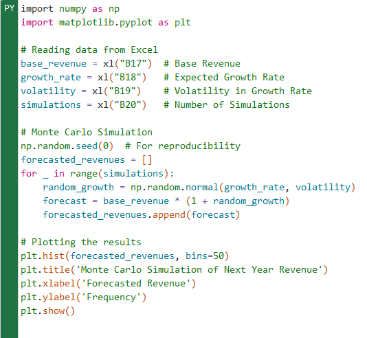
To commit the script, press Ctrl + Enter

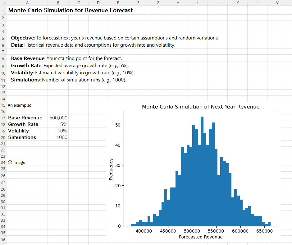
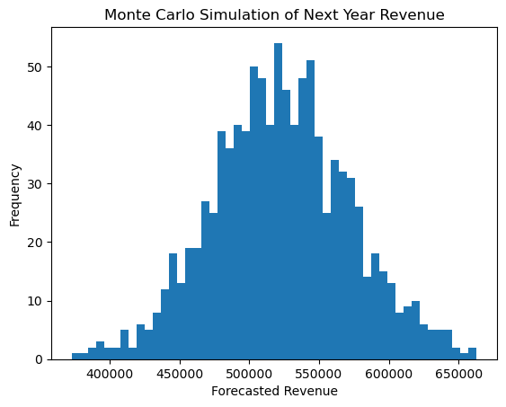
After running the simulations, Python can then plot these outcomes in a histogram, directly from Excel. This histogram visually represents the frequency of different revenue outcomes, giving you a tangible sense of potential future scenarios.

Monte Carlo Simulation Explained

1. np.random.seed(0):
   • This line is used to ensure reproducibility. In random number generation, a 'seed' acts as a starting point. By setting the seed to a specific number (0 in this case), you ensure that every time you run your simulation, you generate the same sequence of random numbers. This is useful for testing and debugging.
2. forecasted_revenues = []:
   • Here, we create an empty list named forecasted_revenues. Think of it as a bucket where we will store all our simulated revenue forecasts.
3. for _ in range(simulations):
   • This line starts a loop that will repeat a certain number of times, equal to the number of simulations you want to run. For instance, if simulations is 1000, the loop will run 1000 times. The _ is a placeholder indicating that we don’t need to use this variable in the loop.
4. Inside the Loop:
   • Each iteration (or run) of the loop simulates one possible future scenario.
   • random_growth = np.random.normal(growth_rate, volatility):
     • This line generates a random growth rate. The function np.random.normal() is used to pick a number from a 'normal' (or 'bell-curve') distribution.
     • growth_rate is the mean (or average) of this distribution — the most likely growth rate.
     • volatility represents the standard deviation, which indicates how spread out the values can be around the mean. A higher volatility means the actual growth rate can vary more significantly from the average.
   • forecast = base_revenue * (1 + random_growth):
     • Now, we calculate the forecasted revenue for this simulation. We take the base_revenue and increase it by the random_growth rate we just generated.
     • 1 + random_growth is used because if, for example, random_growth is 0.05 (or 5%), we want to grow the base_revenue by 5%.
   • forecasted_revenues.append(forecast):
     • Finally, we add (or 'append') the forecasted revenue for this simulation to our list forecasted_revenues.

After the loop finishes running all the simulations, forecasted_revenues will have as many different forecasted values as the number of simulations run. Each value is a potential outcome for next year’s revenue, considering the variability in growth.

Think of this code like playing a video game multiple times (each playthrough is a simulation), and each time you play, the conditions are slightly different (random growth rate). By playing it many times, you get a sense of all the different ways the game could end (forecasted revenues). This helps you understand not just the most likely outcome, but also the range of possible outcomes.

The true power of Monte Carlo Simulation in Excel, powered by Python, lies in its application to real-world financial modeling, particularly in scenario construction. In financial planning and analysis, constructing various scenarios is a critical step to anticipate future outcomes and make informed decisions.

Here's how you can apply this technique in your financial models:

1. Risk Assessment and Decision Making: Use Monte Carlo Simulation to assess the risk of different investment or business decisions. By simulating a wide range of possible outcomes, you can gauge potential risks more effectively and choose strategies that offer the best balance between risk and reward.
2. Budgeting and Forecasting: Incorporate simulations in your budgeting process. For instance, you can forecast revenues, expenses, or cash flows under different market conditions. This approach helps in creating a more robust budget that accounts for uncertainties and potential market fluctuations.
3. Project Valuation: Apply the technique in valuing projects or investments. Monte Carlo simulations can provide a range of values for Net Present Value (NPV) or Internal Rate of Return (IRR), considering the uncertainty in key inputs like discount rates or future cash flows.
4. Scenario Analysis in Strategic Planning: Use the simulations to create multiple economic scenarios (like best case, worst case, and most likely case) in your strategic planning. This will allow you to develop flexible strategies that can adapt to different possible future states of the market or economy.
5. Portfolio Management: For those in asset management or personal finance, apply Monte Carlo Simulation to understand the range of potential future values of an investment portfolio, helping in making more informed investment choices.

By integrating Monte Carlo Simulation into your Excel-based financial models, you can transform static models into dynamic ones that better reflect the complexities and uncertainties of the financial world. This not only enhances your forecasting accuracy but also provides a deeper insight into the potential impact of different variables on your financial outcomes, enabling more strategic decision-making.

Download the Excel File here: